Database Operations with esProc

esProc can retrieve data from databases, write data to them and call databases’ stored procedures. Based on the three basic operations, esProc is well suited to many tasks relating to databases.

1. The process of data analysis and task presentation is:
a. Retrieve data from a database through SQL or stored procedures.
b. Get data from other sources (other databases, texts, hdfs, nosql databases, http data sources, json data sources, etc).
c. Process heterogeneous data uniformly.
d. Provide data for application programs or present data with report forms.

2. Tasks processed in batches that are similar to ETL
The process is similar to task analysis and presentation. Their difference is that data of the last operation is not used for presentation, but is written to other databases or other data sources.

3. Modify the current database in batches
One way is to retrieve data from the current database, process them and write them back to the database; the other is to directly process data of the database through SQL or stored procedures.

Now let’s look at in detail some examples of the three basic operations.
A．Retrieve data from databases. 

 

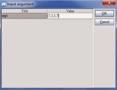
In the above figure, cell A1 has connected to a hsql database named demo. Cell A2 uses SQL statements to query table employee, which is stored in this cell, a variable, as esProc's table sequence; arg1 is a parameter from outside. Cell A3 closes database connection. Cell A4 returns query results outward. In order to make it easier for programmers to write SQL statements, table name and field name of database demo are displayed in the red box in bottom right corner of esProc's integrated development environment.

B．Write data to databases.
esProc can conveniently execute operations of add, delete and update, the simplest code is:
 
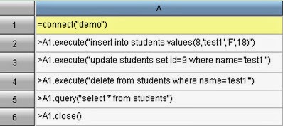
In the above table, insert, update and delete are respectively executed from A2 to A4. Execution of each SQL will be submitted automatically. Note that:
1. It is too frequent access to a database that three SQL statements are submitted three times.
2. There exists no transaction relation between the three SQL statements. So, if the execution of one SQL statement fails, the previous SQL statement remains unaffected.

esProc can update in batches by directly using table sequences. For example: import students’ information from students.txt to update table students1 in the database. Since there are a lot of records to be modified, submitting transactions in batches is more reasonable.
 
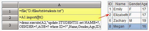
A1：Define a file object in which students’ information is saved.
A2：Import file content.
A3：Use students’ information in A2 to update table students1 in batches. Here submitting SQL in batches can avoid accessing the database too frequently. Meanwhile, this can ensure data consistency, that is, simultaneous success or fail of writing the whole batch of data to the database.

esProc can aslo deal with the complete database transaction consisting of multiple SQL statements. For example, we’ll add a new student, the student’s id should be modified to 9 after data are inserted. In order to ensure data consistency, submission must be executed after the insertion and modification are proved to be successful. Otherwise rollback should be executed.


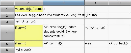
A1：Connect to the database. Note that connect function has used @e option and the subsequent code will return error message when something wrong happens. If the option is not used, the database will terminate esProc program immediately when errors occur.
A2：Execute the insert SQL statement. Note that execute function uses @k option, meaning the transaction will not be submitted automatically after it is executed. If the option is not used, the insert SQL statement will be submitted immediately.
A3：Get the result of last operation in the database, i.e., the insert statement. If err variable is zero, the execution is successful; otherwise, err is the error code.
A4：Judging whether err variable, the execution result, is zero. If the answer is yes, the last operation of the insert statement is successful and modification in B4 can be executed.
C4：Get execution result of update SQL.
A5：Make judgment over variable err. If it is zero, submit the database; otherwise execute rollback.
A6：Close database connection.

C．Call stored procedures

For stored procedures that don’t return parameters, esProc's method of calling them is simple:
 
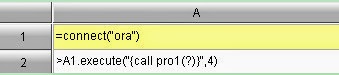
A1：Connect the database.
A2：Call the stored procedure, value of output parameter is 4.

esProc call stored procedures with result sets in this way:
 
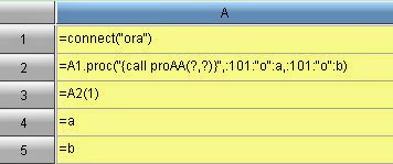
Cell A2 uses proc function to call the stored procedure: orac.proc("{call proAA(?,?)}",:101:"o":a,:101:"o":b). It returns two result sets (table sequences) to form a sequence, i.e., a set of table sequence, which assigns value to A1. The following is to explain proc function’s input parameters one by one.
1) SQL strings
"{call proAA(?,?)}" contains name of the stored procedure to be called, the question marks represent SQL's parameters.
2) Output parameter 1
:101:"o":a defines an output parameter in which 101 represents that its data type is cursor ( for other types, please see appendix) and ”o” represents that it is an output parameter. a defines a variable by which returned results can be referenced.
3) Output parameter 2
:101:"o":b defines an output parameter in which 101 represents that that its data type is cursor and "o" represents that it is an output parameter. b defines a variable by which returned results can be referenced.
Cell A3 returns cell A2's first table sequence (table emp's result set).
Cell A4 and A5 use output variables a and b respectively in A2 to get the execution results corresponding to the stored procedure. a corresponds to data of table emp and assigns value to A3; b corresponds to data of table test and assigns value to A4.

Appendix: Definition of Parameter Type
Values of type are:
public final static byte DT_DEFAULT = (byte) 0; // by default, identify automatically
public final static byte DT_INT = (byte) 1;
public final static byte DT_LONG = (byte) 2;
public final static byte DT_SHORT = (byte) 3;
public final static byte DT_BIGINT = (byte) 4;
public final static byte DT_FLOAT = (byte) 5;
public final static byte DT_DOUBLE = (byte) 6;
public final static byte DT_DECIMAL = (byte) 7;
        public final static byte DT_DATE = (byte) 8;
public final static byte DT_TIME = (byte) 9;
public final static byte DT_DATETIME = (byte) 10;
public final static byte DT_STRING = (byte) 11;
public final static byte DT_BOOLEAN = (byte) 12;

public final static byte DT_INT_ARR = (byte) 51;
public final static byte DT_LONG_ARR = (byte) 52;
Publicfinal static byte DT_SHORT_ARR = (byte) 53;
public final static byte DT_BIGINT_ARR = (byte) 54;
public final static byte DT_FLOAT_ARR = (byte) 55;
public final static byte DT_DOUBLE_ARR = (byte) 56;
public final static byte DT_DECIMAL_ARR = (byte) 57;

public final static byte DT_DATE_ARR = (byte) 58;
public final static byte DT_TIME_ARR = (byte) 59;
public final static byte DT_DATETIME_ARR = (byte) 60;
public final static byte DT_STRING_ARR = (byte) 61;
public final static byte DT_BYTE_ARR = (byte) 62;
public final static byte DT_CURSOR = (byte) 101;
public final static byte DT_AUTOINCREMENT = (byte) 102;

Examples of Database Transaction Management with esProc

esProc can write to databases and manage database transactions. Here we'll look at the programming method of rollbacks and controlling transaction submission, etc. 

A．Submit transactions automatically

esProc can conveniently execute operations like insert, delete and update. The simplest code is:

 

In the above figure, insert, update and delete are respectively executed from A2 to A4. Execution of each SQL statement will be submitted automatically. Note that:

1. That three SQL statements are submitted three times is too frequent operations for a database. 

2. There exists no transaction relation between the three SQL statements. So, if the execution of one SQL statement fails, the previous SQL statement will remain unaffected. 

The following examples are to introduce how to submit transactions in batches and how to compose a transaction with multiple SQL statements in a table sequence. 

B．Submit transactions in batches

Import students' information from students.txt to update table students1 in the database. Since there are a lot of records to be modified, using method of submitting transactions in batches is more reasonable. 

 

A1：Define a file object in which students’ information is stored. 

A2：Import file content. 

A3：Use students’ information in A2 to update table students1in batches. Submitting SQL in batches can avoid accessing the database too frequently. Meanwhile, this can ensure consistency of the data for the submission could succeed or fail simultaneously. 

C．Program control transactions

Now we’ll add a new student. The student’s id should be modified to 9 after data are inserted. In order to ensure consistency of the data, submission must be executed after the insertion and modification are proved to be successful. Otherwise rollback should be executed.

 

A1：Connect to the database. Note that connect function uses option @e and the subsequent code will return error message when something wrong happens. If the option is not used, the database will terminate esProc program directly when errors occur.  

A2：Execute the insert SQL statement. Note that execute function uses option @k, meaning the transaction will not automatically submitted after it is executed. If the option is not used, the insert SQL statement will be submitted immediately. 

A3：Get the result of last operation in the database, i.e., the insertstatement. If err variable is zero, the execution is successful; otherwise, err is the error code. 

A4：Judging whether err variable, the execution result, is zero. If the answer is yes, the last operation of the insert statement is successful and modification in B4 can be executed.

C4：Get execution result of the update SQL. 

A5：Make judgment over err variable. If it is zero, submit the database; otherwise execute rollback.  

A6：Close database connection.

A Code Example of Computing Link Relative Ratio and Year-on-year Comparison with esProc

Link relative ratio refers to comparison between the current data and data of the previous period. The interval is usually one month. For example, divide sales amount of April by that of March, and you get the link relative ratio of April. Hour, day, week and quarter can also be used as the time interval. Year-on-year comparison is the comparison between the current data and data of the corresponding period of the previous year. For example, divide sales amount of April 2014 by that of April 2013. In business, data of multiple periods is usually computed to find the variation trend.
Seeking link relative ratio and year-on-year comparison is common inter-row and inter-group computations, which are easy to be performed with esProc. The following example is used to illustrate the computations.

Case description

Compute link relative ratio and year-on-year comparison of each month’s sales amount within the designated period. The data comes from table order. Some of the data is shown below:

esProc:
   A1=esProc.query("select * from sales3 where OrderDate>=? and       OrderDate<=?",begin,end)
   A2=A1.groups(year(OrderDate):y,month(OrderDate):m;sum(Amount):mAmount)
   A3=A2.derive(mAmount/mAmount[-1]:lrr)
   A4=A3.sort(m)
   A5=A4.derive(if(m==m[-1],mAmount/mAmount[-1],null):yoy)

Code interpretation:
A1: Query in the database according to periods. begin and end are external parameters. Such as, begin="2011-01-01 00:00:00", end="2014-07-08 00:00:00"(i.e. the date of today which can be obtained through now() function). Some of the query results are as follows:
 

A2: Group orders by year and month, then summarize and seek each month’s sales amount. Some of the computed results are as follows:
 

A3: Add a new field Irr, i.e, the link relative ratio on a month-on-month basis. The code is mAmount/mAmount[-1], in which mAmount represents sales amount of the current month, and mAmount[-1] represents that of the previous month. Note that the initial month’s link relative ratio is empty (i.e. January 2011). Computed results are:
 

A4: Sort A3 by month and year to compute year-on-year comparison. Complete code should be: =A3.sort(m,y). Since A3 is originally sorted by the year, so we just need to sort by the month, the code is: A3.sort(m), which has a higher performance. Some of the computed results are:
 

A5: A5: Add a new field yoy, i.e., theyear-on-year comparison of monthly sales amount. The code is: if(m==m[-1],mAmount/mAmount[-1],null), meaning that the computation of year-on-year comparison is only performed over the corresponding months. Note that the year-on-year comparison for months of the initial year (i.e. the year 2011) is always. Some of the computed results are:  
 

A row of code, A6=A5.sort(y:-1,m), can be added to make observation easier. That is, sort A5 in descending year order and ascending month order. Note that the data comes to an end in July 2014. Results are shown below:
 

Code Examples of Common In-Memory Grouping with esProc

It is convenient to realize some common in-memory grouping with esProc, such as, equal grouping, alignment grouping and enumeration grouping. They are to be illustrated with the following examples.

Equal grouping 

Grouping basis of equal grouping is certain fields (or computed columns derived from fields) within a data set. Each group is a subset of original data set.

Case description: Group sales orders by the year. 

Data description: Data of sales orders are shown below: 

The above data set (table sequence) can be accessed from a database or a file.

For example:     A1=file("E:/sales.txt").import@t()

esProc: A2=A1.group(year(OrderDate))

Computed results:

 

Code interpretation:

1. In this example, grouping basis comes from OrderDate. The date of sales order will be converted into the year through year(OrderDate), and data of the same year will be grouped together. 

2. There may be multiple fields for grouping. For example, regroup data of different years and sellers according to year and sellers. The code is: 

A1.group(year(OrderDate),SellerId)

3. Often, the grouped data are used to perform aggregation operations, such as, compute each year’s sales amount according to A2. The code is:

A2.new(year(OrderDate):y,~.sum(Amount):a)

Computed results are:

 

Or, combine grouping and summarizing into one step with groups function:

A1.groups(year(OrderDate):y; sum(Amount):a)

Of course, sometimes we have to execute grouping and summarizing separately in order to reuse the code and improve computational efficiency. For example, filter one of the groups of A2, and perform association computation for another group. Another situation is that, if, after summarizing, data of a certain group are unusual and worth further study, then this group can be used directly to go on with the computations. It’s no need to filter the group again.   

4. By default, esProc's group function will group data by using hash algorithm. But, comparing adjacent rows can have higher performance for ordered data. This can be executed by using option @o in group function. For example: 

A1.group@o(year(OrderDate),SellerId)

Alignment grouping

Criterions used for equal grouping come from within a dataset. But sometimes, they originate from without, like fields of other data sets, arrays created by users, parameter list and so on. Thus the alignment grouping comes into being. 

Different from equal grouping, method of alignment grouping may produce empty subsets, which have no members to correspond to data of a group. It may also produce incomplete groups, meaning that some data won’t be included in any group. These things won’t happen for equal grouping.  

Case description: Table of top 10 sellers has been worked out in the light of performance, please group sales orders according to the table order. 

The data set before grouping: 

The sales orders are the same as those in above example. Data are stored in A1.

Table of the top 10 sellers is stored in B1 as follows: 

 

Sellers table may come from a temporary table, or be generated by a piece of code. The generating process is not the focus of this example. 

esProc:   A1.align@a(B1:empID,SellerId)

Computed results:

 

Code interpretation:

1. In this example, the grouping basis (sellers table) comes from without the data set to be grouped. After grouping is completed, a group contains only the data of one seller, and groups are sorted according to sellers table.  

2. Because sellers in sales orders outnumber those in sellers table, some of the orders won’t appear in any groups. If we want to create one more group to store these orders, we can use function option @n as follows: 

A1.align@a@n(B1:empID,SellerId)

The one more group will be put last as follows:  

 

3. Sometimes, the grouping basis is not within the data set to be grouped, such as, “newly-employed sellers table”. In this case, it’s normal to produce empty groups. Modify the first group of data in the table into empID=100, for example, the computed results will be: 

Enumeration grouping  

The grouping basis for enumeration grouping could be more flexible. It could be any Boolean expressions. Those records consistent with the expression will get into the same group. 

Similar to alignment grouping, enumeration grouping is also of incomplete grouping, probably producing empty subsets or results that some records are not included in any group. In addition, with this grouping method, it is likely that some records may appear in more than one group.

Case description: Divide sales orders into four groups, they are: A. order amount is less than 1000; B. order amount is less than 2000; C. order amount is less than 3000; D. order amount is less than 10,000. Note that the data cannot be grouped repeatedly, that is, if an order has been in group A, it must not be put into group B, C, or D. 

The data set before grouping: 

The sales orders are the same as those in above example. Data are stored in A1. 

esProc code:

  A2=["?<=1000","?<=2000","?<=3000","?<=10000"]

A3=A1.enum(A2,Amount)

Computed results:

 

Case interpretation: 

1. In this example, grouping basis for grouping is multiple flexible expressions. Each record will be compared with the expressions. Those consistent with the same expression will be put into the same group. Groups are sorted according to order of grouping basis as well.

2. By default, enumeration grouping will not produce identical results. The method, which is showed in the above example, is that after group A’s data are selected, the rest of data will be compared with expression B to see their consistency. While the use of function option @r, which represents that all data are compared with expression B, may produce identical results. For example: A3=A1.enum@r(A2,Amount), computed results are: 

 

3. Similar to alignment grouping, if the expression for enumeration grouping is inconsistent with any data to be grouped, empty group will appear. Besides, if some data are inconsistent with any expression, function option @n can be used to put them into a surplus group. 

Code Examples of Calling Database Stored Procedures in esProc

esProc can call database stored procedures conveniently. This article will illustrate in detail the program writing with examples.

A.Call stored procedures without return values

 Take oracle stored procedure as an example, the stored procedure has only one input parameter, and no output parameter: 

    create or replace procedure pro1

    (pid IN VARCHAR)

    as

    begin

    insert into emp values(pid,'mike');

    update emp set name='rose' where id=pid;

    commit;

    end;

execute function or proc function can be used in esProc to call this stored procedure:

A1：Connect to the database.

A2：Call stored procedure, input parameter value is 4.

proc function is mainly used to call stored procedures which return values and result sets, or to call stored procedure pro1 which does not return parameters. 

A1：Connect to the database.

A2：Call stored procedure pro1. The code 4:0:"i": after comma describes and defines an input parameter, in which 4 is the input parameter value, 0 represents that the type of input parameter is automatically identified by esProc, and "i" represents input type. If the parameter type need to be designated manually, the code may be written as 4:1:"i":, in which the 1 in the middle represents Integer(int). For more information about parameter types supported by esProc, please see appendix: Definition of Parameter Types.

B. Call stored procedures which return a single value

The stored procedure below will return one parameter value, so proc function, instead of execute function, will be used.

    create or replace procedure testb

    (para1 in varchar2,para2 out varchar2)  

    as

    begin

    select name into para2 from emp where id= para1;

    end testb;

The code for calling this stored procedure by esProc is:

A1：Connect to the database.
A2：proc function is used to call stored procedure testb. Here two parameters are used: one is 1:0:"i" representing that the value is 1 and the input parameter is automatically identified; the other is 11:"o":name in which 11 represents string type (see appendix Definition of Parameter Types for more), "o" represents type of output parameter and name defines an esProc variable to receive return values for the output parameter.
A3：Assign output value of stored procedure in A2 to cell A3 through name variable.

C. Call stored procedures which return a single result set
    Stored procedure RQ_TEST_CUR returns a single result set
    CREATE OR REPLACE PROCEDURE RQ_TEST_CUR
    (
V_TEMP OUT TYPE.RQ_REF_CURSOR,
PID IN VARCHAR
    )
    AS
    BEGIN
OPEN V_TEMP FOR SELECT * FROM TEST WHERE ID =PID;
    END RQ_TEST_CUR;

The stored procedure has an input parameter and returns a result set. The code for calling the stored procedure in esProc is as follows:

Cell A2 uses proc function to call the stored procedure: proc("{call RQ_TEST_CUR(?,?)}",:101:"o":table1,1:0:"i":). The following will explain the input parameters of proc function.
1） SQL strings
"{call RQ_TEST_CUR(?,?)}" represents calling the stored procedure’s name. The question marks represent SQL's parameters.
2） Output parameters
:101:"o":table1 defines an output parameter, in which 101 represents that its data type is cursor, and ”o” represents that it is an output parameter. Table1 defines a variable which is used to reference returned results. 1:0:"i": defines an input parameter, in which 1 is value of the input parameter, 0 represents that the parameter type is automatically identified by esProc.
Cell A3 uses output variable in A1 to reference the execution results of the stored procedure. Computed result is a table sequence containing two fields: id and name, which is the same as that in A2.

D. Call stored procedures which return multiple result sets
The code will begin with an oracle stored procedure which returns two result sets:
    create or replace procedure proAA
    (
out_var out sys_refcursor,
out_var2 out sys_refcursor
    )
    as
    begin
openout_var for select * from emp;
open out_var2 for select * from test;
    end;
The stored procedure returns result sets of two tables: emp and test. Call the stored procedure in esProc and the program for receiving the two result sets is as follows:

Cell A2 uses proc function to call the stored procedure: orac.proc("{call proAA(?,?)}",:101:"o":a,:101:"o":b), which returns two result sets (table sequences) to form a sequence, i.e., a set of table sequence. The sequence assigns value to A2. The following will explain the input parameters ofproc function.
1）SQL strings
"{call proAA(?,?)}" represents calling the stored procedure’s name. The question marks represent SQL's parameters.
2）Output parameter 1
:101:"o":a defines an output parameter, in which 101 represents that its data type is cursor, and "o" represents it is an output parameter. a defines a variable which is used to reference returned results.
3）Output parameter 2
:101:"o":b defines an output parameter, in which 101 represents that its data type is cursor, and "o" represents it is an output parameter. b defines a variable which is used to reference returned results.

Cell A3 returns cell A2’s first table sequence (table emp's result set)
Cell A4 and cell A5 use respectively the output variables a and b in A2 to obtain execution results of corresponding stored procedure. a corresponds to data in table emp and assigns value to A4; b corresponds to data in table test and assigns value to A5.

Appendix: Definition of Parameter Types
Values of type are:
public final static byte DT_DEFAULT = (byte) 0; //default, automatically identify
public final static byte DT_INT = (byte) 1;
public final static byte DT_LONG = (byte) 2;
public final static byte DT_SHORT = (byte) 3;
public final static byte DT_BIGINT = (byte) 4;
public final static byte DT_FLOAT = (byte) 5;
public final static byte DT_DOUBLE = (byte) 6;
public final static byte DT_DECIMAL = (byte) 7;
        public final static byte DT_DATE = (byte) 8;
public final static byte DT_TIME = (byte) 9;
public final static byte DT_DATETIME = (byte) 10;
public final static byte DT_STRING = (byte) 11;
public final static byte DT_BOOLEAN = (byte) 12;

public final static byte DT_INT_ARR = (byte) 51;
public final static byte DT_LONG_ARR = (byte) 52;
public final static byte DT_SHORT_ARR = (byte) 53;
public final static byte DT_BIGINT_ARR = (byte) 54;
public final static byte DT_FLOAT_ARR = (byte) 55;
public final static byte DT_DOUBLE_ARR = (byte) 56;
public final static byte DT_DECIMAL_ARR = (byte) 57;

public final static byte DT_DATE_ARR = (byte) 58;
public final static byte DT_TIME_ARR = (byte) 59;
public final static byte DT_DATETIME_ARR = (byte) 60;
public final static byte DT_STRING_ARR = (byte) 61;
public final static byte DT_BYTE_ARR = (byte) 62;
public final static byte DT_CURSOR = (byte) 101;
public final static byte DT_AUTOINCREMENT = (byte) 102;

Control of Database Connection in esProc

In handling database transactions, some operations may cause errors, which may bring about unpredictable results, especially in batch processing. In order to avoid this situation, database connection should be under control and error messages should be handled appropriately.

1. Database error messages
Let’s study database error messages first. Use an Access file DbCon.accdb as the target database, and create an ODBC data source in esProc. Use data of the file directly and write a connection string in the ODBC data source:DRIVER=Microsoft Access Driver (*.mdb, *.accdb);DBQ=D:\\files\\DbCon.accdb：

An empty table CityBak was created in the Access file DbCon.accdb:

 
In the table, ID is the primary key, and especially, data of POPULATION should be>1000000.

Now prepare to write CITIES' data in database demo to table CityBak:  


A1 gets table CITIES’s data from database demo:
 

A2 connects to database DbCon. A3 gets data from table CityBak; since it is a newly-created table, there are no records in it. 
 

An error occurs in A4. Because of the criterion POPULATION>1000000, the execution of writing the tenth record of Detroit's information to the database fails. By default, the execution will be terminated when errors occur in database operations. 
But we can look up the data-writing result in another dfx:

Query results of A2 are as follows: 
 
It can be seen that some of the data has been written to the target table successfully though the execution of program in the first cellset failed due to data constraint in table CityBak. 
Once database errors occur while updating a database in batches,program will be terminated. In order to avoid this situation, @e option can be used at the beginning of connecting to handle the errors manually while the connection remains. For example:

@e option is used in A2 when the database connection is established, so the code can respond manually to possible errors. In order to keep consistent with the preceding query results, the existing records in table CityBak should be emptied in A2 first. Thus query results of A5 will be the same with the preceding ones:
 



Because there were operations disagreeing with data constraint when updating table CityBak's data in A4, error code can be found in B4:
 
It should be noted that once database errors occur while batch updating a database, the updating will stop and errors will be recorded. By modifying the expression in A4 to =A2.error@m(), we can see the error messages:

We'll make further study: 

Using @a option indb.update@a() can empty database table before updating, then it is unnecessary to add statements to delete records. Get the first 5 records in A3 and write them to CityBak. Now since all the records satisfy the data constraint, the statements execution in A3 goes well and the error code in B3 is zero:
 
In A5, the records are stored successfully: 

2.Control of submission and rollback
We cannot know beforehand whether the batch update of records is successfully completed or not, and which records may go wrong. By default, each record’s update will be automatically submitted, which makes the results unpredictable. This is far from ideal for database management. 

In handling database transactions, sometimes we need to decide whether we should submit the update to the database or cancel the execution, as appropriate. In this circumstance, we use db.commit() and db.rollback() to take control.

The executed statements in esProc are by default submitted automatically and thus,out of control. If we want to use db.commit() and db.rollback() to control the submission, @k option is needed in executing statements to make code has control of the submission. In this way, we can decide if the data are eligible in the light of error messages. In the following example, all data become ineligible if there is something wrong with the batch update. This can prevent unpredictable results in the database:

A3 empties table CityBak and executes submission automatically because it didn't use @k option when executing db.execute(). 

Errors may occur in A4 when executing batch update, which can be seen in A5's computed result: 
 
Therefore, rollback in B6 will be executed and data won’t be written to the database. Query results of A7 are as follows: 
 
We can see according to error code that all goes well when executing batch update with @k option, like the executed statements in A8. Value of A9 is: 
 
Now submission in B9 will be executed and data will be written to the database. Query results of A11 are as follows:
 

Program 24-Point Calculation with esProc

24-point calculation is a common intellectual game, which can be played with poker without jokers. Draw four cards randomly, use the four numbers to work out 24 points with four arithmetic operations: addition, subtraction, multiplication and division. In playing poker, JQK usually correspond numbers 11, 12 and 13.

With esProc, we could program the game more conveniently. Working out a solution with four random numbers becomes easier:

Let’s analyzes the piece of code in detail.

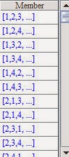
Four numbers for computation are given in A1. First, we try all possible permutations of the four random cards. To do this, we list the repeatable cases in A2 with the help of a four-digit base-4 number. In B2, we only select those cases which are not repeated. See figure below:
 
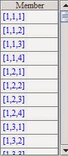
Any three symbols of four arithmetic operations need to be inserted in computation. Each symbol is selected arbitrarily among plus, minus, times and division. Execute in A3 the loop of a three-digit base-4 number, and list all possible combinations:
 
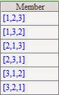
Different computation orders have different computed results. The computing order can be changed by adding brackets. Three operational symbols show that the computation can be divided into three steps, and brackets adding decides the execution order of the three steps. Combinations in B3, selected from the results in A3,contain all three elements 1,2,3, and represent all possible execution orders. See figure below:
 
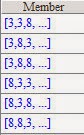
Since there could be repeated numbers among the four randomly selected cards, all permutations of cards will be listed in A4 and remove those repeated ones in B4 in order to avoid redundant loop. Let’s look at [8,3,8,3] in A1, its eligible combinations are as follow:
 
For each permutation, the programming in line 5 and line 6 executes loop of every symbol selection and every computation order. Then computes by calling subprogram in A8 and with the copied parameters to avoid interfering the subsequent computation.

When the subprogram in A8 is called, numerical sequence, symbol sequence, and sequence of computation order should be filled respectively into A8, B8 and C8; at the same time, expression for computation should be prepared in D8. B9 executes the loop of sequence of computation order until the result is gradually obtained. C9 gets the result of a single step by calling subprogram in A13. The subprogram, which is quite simple, achieves computed results of four arithmetic operations based on two given numbers and one of the symbols. D9 aims at the expression used for single step computing, after which the original two numbers will become one, and expression sequence, symbol sequence and numerical sequence will be modified in E9, C10 and D10. Having done the single step computing, the original total computing steps will be reduced by one, so another modification of sequence of computation order will be required in E10. In line 11, unless it is the last step, brackets will be added to newly-created expression to ensure an appropriate computing order.

When the loop in B9 is over, subprogram in A8 completes its computation of expression for this case. B18 is programmed to decide whether the result is 24. The result will be calculated to three decimal places in consideration of computational error of double-precision number. If the result equals to 24, the current permutation is eligible. The corresponding expression will be put in B1 in C12.

If the loop of all conditions is finished, yet no expression is found in B1 when checking A7, no solution has been obtained.
After all the computation, result can be found in B1. See below:
 
Or cellset parameter will take the place of combination of numerical value entered in A1:


Set cellset parameter before doing computation:
 
The result displayed in B1 after computation is as follow: