How to Compute Moving Average in R Language

A moving average is used to smooth out a time series. Computing moving average is a typical case of ordered data computing. Its basic computing method is to create a subset composed of N consecutive members of a time series, compute the average of the set and shift the subset forward one by one. The following example teaches you how to compute moving average in R language.

Case description:

Data frame sales has two fields: salesDate and Amount of this date. Requirement: compute the moving average in three days. Computing steps include seeking sales amount average of the previous day, the current day and the next day, and shift forward along the dates. A part of the source data is as follows:

Code:

  filter(sales$Amount/3, rep(1, 3))

Computed result:

Code interpretation:

filter function can be used in R language to compute moving average, which produces concise code. This method is quite convenient.

Despite the convenience of the filter function, it is difficult to understand for beginners. For example, sales$Amount/3 means dividing the current value of field Amount by three,but when it is used in filter function, it may mean adding the three consecutive values together, then divide the sum by three. [1,1,1] is the value of expression rep(1,3), which is used here to specify the range of data fetching. In addition, because neither the name nor the parameters of filter function contain the words "average" and "moving", even many developers of R language don't know its use for computing moving average.

In fact, filter function is a universal linear filter. Its use is more than computing moving average. Its complete function reference is filter(x, filter, method = c("convolution", "recursive"),sides = 2, circular = FALSE, init).

Any modification of the requirement will make the code more difficult to understand. For example, the code for computing moving average of the current day and the previous two days cannot be written as filter(sales$Amount/3, rep(0,2)), it has to befilter(sales$Amount/3, rep(1,3), sides = 1).

Summary:

R language can compute moving average, but its code is rather elusive.

Third-party solutions

We can also use Python, esProc and Perl to handle this case. As R language, all of these languages can perform data statistics and analysis and compute moving average. The following introduces solutions of Python and esProc briefly.

Python(pandas)

Pandas is Python's third-party library function. It is powerful in processing structured data with basic data type imitating R's dataframe. At present the latest version is 0.14. Its code for handling this case is as follows:

   pandas.stats.moments.rolling_mean(sales["Amount"], 3)

The name of rolling_mean function is clear, even a developer without experience with pandas can understand it easily. The function’s usage is simple too. Its first parameter is the sequence being computed and the second parameter is N, which is the number of days in seeking moving average.

esProc

esProc is good at expressing business logic freely with agile syntax. Its expressions for relative position can solve computational problems of ordering data easily. The code is as follows:

   sales.(Amount{-1,1}.avg())

{-1,1} in the code represents a relative interval, that is, the three days of the previous day, the current day and the next day. It can be seen that moving average can be worked out clearly and flexibly by using a relative interval. If it is required, for example, to compute the moving average of the current day and the previous two days, we just need to change the interval to {-2,0}in esProc.

A relative interval is a set. esProc can also express an element of relative position. For example, it can compute sales growth rate with (Amount -Amount[-1]) conveniently. In contrast, the code in R language and Python is difficult to understand. 

Set Operators in esProc

Since sets are commonly used in esProc, the latter provides comprehensive set operations.

1. Binary Operation on Sets

The most basic set in esProc is sequence. Let's look at some basic binary operations between two sequences A and B.

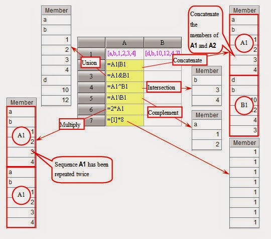
Ø  A|B

Concatenate: Concatenate the two sequence straightforwardly, of which the member of B is added behind the members of A. If A or B or both A and B are the single-value member instead of sequence, then it will be handled as a single member sequence.

Ø  A&B

Union: Join the two sets and remove the members of B that already exist in A. If one of A and B or both vales are the single-value member instead of sequence, then you can take it as single member sequence to process.

Ø  A^B

Intersection: Intersection set of A and B. Get a sequence composed of members that not only exist in A but also exist in B.

Ø  A\B

Complement: Members in A but not in B. If B is not a sequence, then treat it as the single member sequence.

Ø  k*A

A|A|…|A, copy A for k times, positions of k and A are interchangeable in the expression.  

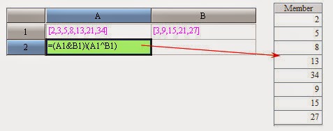
These basic operations - concatenate, complement, intersection and union - can also be used to deal with more complex set operations. Such as, to seek the “inverse intersection” of sets A and B, i.e., the set composed of all that is not the common members of A and B. 
The "inverse intersection" of two sets is the complement of their union and intersection. With this kind of transformation, more complex binary operations will be completed.

2 Alignment Arithmetic Operation on Sets

Two sequences which have the same length will perform the alignment computation on members, and return a new sequence.

Ø  A++B

[A(1)+B(1),A(2)+B(2),…]

Ø  A--B

[A(1)-B(1),A(2)-B(2),…]

Ø  A**B

[A(1)*B(1),A(2)*B(2),…]

Ø  A//B

[A(1)/B(1),A(2)/B(2),…]

Ø  A%%B

[A(1)%B(1),A(2)%B(2),…], the % here is the Mod computation.

Ø  A\\B

[A(1)\B(1),A(2)\B(2),…], the slash here means integer division

3. Comparison of Sets

In esProc, the function cmp(A,B) can be used to compare the sequence A and B.

Ø  cmp(A,B)

Compare the member values of two sequences at the same location one by one, and return the 1 or -1 when encountering the first unequal member, if A is identical to B, then return 0. Specifically, cmp(A) or cmp(A,0) will compare A with the sequence with the same length and members are all 0, i.e. cmp(A,[0,0,…,0]).

Comparison of two sequences can be briefly expressed as A==B, A>B.

Note that a sequence in esProc is an ordered set, so order plays an important role in comparing the size of two sequences A and B. A.eq(B) is used to see if the two sequences have common members. 

Because the member order in A1 and A2 is different, result in A3 is false, showing the two sequences are not equal. While result in A4 is true, showing the two sequences have the same members. 

The Disadvantages of SQL Computation (I)

SQL is invented primarily to provide a method to access structured data in order to transparentise the physical storage scheme, so a lot of various types of English vocabularies and syntaxes are used in SQL to reduce the difficulty in understanding and writing it. And the relational algebra as the basic theory of SQL is a complete computation system, which can compute everything in principle. In terms of this, we certainly should use SQL to satisfy various demands for data computation.

But, though relational database has achieved a huge success, evidently SQL fails to realize its original aim of invention. Except very few simple queries can be completed by end user using SQL, most of SQL users are still technical personnel, and even many complex queries are no easy job for technical personnel.

Why? We inspect the disadvantage of SQL in computation through a very simple example.

Suppose there is a sales performance table consisting of three fields (to simplify the problem, date information is omitted):

sales_amount	Sales performance table
sales	Name of salesman, suppose there is no duplicate name.
product	Products sold
amount	Sales amount of the salesman on the product

Now we want to know the name list of the salespersons whose sales amounts rank among the top 10 places both in air-conditioners and TV sets.

This question is rather simple and people will very naturally design out the computation process as follows:

1) Arrange the sequence according to the sales amount of air-conditioner and find out the top 10 places.

2) Arrange the sequence according to the sales amount of TV and find out the top 10 places.

3) Get the intersection of the results of 1 and 2 and obtain the answer.

   

Now we use SQL to do it.

1) Find out the top 10 places of the sales amount of air-conditioner. This is very simple:

select top 10 sales from sales_amount where product='AC' order by amount desc

2) Find out the top 10 places of the sales amount of TV. The action is the same:

select top 10 sales from sales_amount where product='TV' order by amount desc

3) Seek the intersection of 1 and 2. This is somewhat troublesome, as SQL does not support computation by steps. The computation result of the above two steps cannot be saved, and thus it is necessary to copy it once again:

select * from

( select top 10 sales from sales_amount where product='AC' order by amount desc )

intersect

( select top 10 sales from sales_amount where product='TV' order by amount desc )

A simple 3-step computation has to be written like this using SQL, and daily computations of more than 10 steps are in great numbers. So this evidently goes beyond the acceptability of many people.

In this way, we know the first important disadvantage of SQL: Do not support computation by steps. Dividing complex computation into several steps can reduce the difficulty of a problem to a great extent. On the contrary, completing many steps of computation into one step can increase the difficulty of a problem to a great extent.

It can be imagined that, if a teacher requires pupils to create only one calculation formula to complete the calculation in solving application problems, how distressed the pupils will feel (of course, there are certain clever children who can solve the problem)!

SQL query cannot by conducted by steps, but the stored procedure written out with SQL can operate by steps. Then, is it possible to use the stored procedure to conveniently solve this problem?

For the time being, we just ignore how complex is the technical environment in which the stored procedure is used (this is enough to make most people give it up) and the incompatibility caused by differences of databases. We only try to know theoretically whether it is possible to use SQL to make this computation simpler and faster.

1) Compute the top 10 places sales amount of air-conditioners. The statement is still the same, but we need to save the result for use by Step 3, while in SQL, it is only possible to use table to store set data. So we need to create a temporary table: 

create temporary table x1 as

select top 10 sales from sales_amount where product='AC' order by amount desc

2) Compute the top 10 places of the sales amount of TV. Similarly

create temporary table x2 as

select top 10 sales from sales_amount where product='TV' order by amount desc

3) Seek the intersection, the preceding steps are troublesome but this step is simpler.

select * from x1 intersect x2

After the computation is done in steps, the working thought becomes clear, but it still appears over-elaborate to use a temporary table. In the computation of mass structured data, temporary set, as intermediate result, is rather common. If the temporary table is created for storage in all cases, the computation efficiency is low and it is not intuitive.

  

Moreover, SQL does not allow the value of a certain field to be a set (namely temporary table), so in this way, it is impossible to implement some computations even if we tolerate the over elaborate.

If we change the problem into computing the salespersons whose sales amounts of all products rank among the top 10 places, try thinking how to compute it. By continuing to use the above-mentioned working thought, it is very easy to get the below points:

1) Group the data according to products, arrange the sequence of each group, and get the top 10 places;

2) Get the intersection of the top 10 places of all products; 

As we do not know beforehand how many products there are, so it is necessary to also store the grouping result in a temporary table. There is a field in this table that needs to store the corresponding group members, which is not supported by SQL, so the method is unfeasible.

If supported by window function (SQL2003 standard), it is possible to change the working thought. After grouping by product, compute the number of times each salesman appears in the top 10 places of the sales amounts of all product category group. If the number of times is the same as the total number of the product categories, it indicates this salesman is within the top 10 places regarding the sales amounts of all product categories.

select sales

from ( select sales,

       from ( select sales,

              rank() over (partition by product order by amount desc ) ranking

              from sales_amount)

      where ranking <=10 )

group by sales

having count(*)=(select count(distinct product) from sales_amount)

How many people can write such complex SQL?

Moreover, in many databases, the window functions are not supported. Then, it is only possible to use the stored procedure to develop a loop, according to the sequence, the top 10 places of each product, and seek the intersection of the result of the preceding time. This process is not very much simpler than using high level language to develop, and it is also necessary to cope with the triviality of the temporary table.

Now, we know the second important disadvantage of SQL: Set-lization is not complete. Though SQL has the concept of set, it fails to provide set as a kind of basic data type, which makes it necessary to transform a lot of natural set computations in thinking and writing. 

Structural Data Computing in Java for Non-database

In Java, implementing via SQL is a well-developed practice for database computation. However, the structured data is not only stored in the database, but also in the text, Excel, and XML files. Considering this, how to compute appropriately regarding the structured data from non-database files? This article raises 3 solutions for your reference: implement via Java API, convert to database computation, and adopt the common data computation layers.

Implement via Java API. This is the most straightforward method. Programmers will benefit from Java API in controlling every computational step meticulously, monitoring the computed result in each step intuitively, and debugging conveniently. Needless to say, no learning cost is also an additional advantage of Java API.

Thanks to the well-developed API for retrieving and writing-back data to Txt, Excel, and XML files, Java has enough technical strength to offer the full support for such computation, in particular the simple computational goals.

However, this method requires great workload and quite inconvenient. For example, since the common data algorithms have not implemented in Java, programmers will have to spend great time and efforts to implement all the ins and outs manually by aggregating, filtering, grouping, and sorting and some other common actions. For another example of data storage and detail data retrieval through Java API, programmers will have to combine every data and 2D table with List/map and other objects, and then compute in nested loops at multi-levels. Moreover, such computation usually involves the set operations and relational computations on massive data, as well as the computations between objects and object properties. It takes great efforts to implement the underlying logics and even greater workload in handling the complex ordered computation.

In order to reduce the programming workload, programmers always prefer leveraging the existing algorithms to implementing all specifics by themselves. In view of this, the second choice below would be a better choice:

        

Convert to database computation.This is the most conservative method. Concretely speaking, it is to import the non-database data to the database via the common ETL tools like DataStage, DTS, Informatica, and Kettle. The advantages of this practice include the high computational efficiency, steadfast running, and less workload for Java programmers. It fits for the scenarios of great data volume, high performance demand, and medium-level computational complexity. These advantages are evident for the mixed computation on the database and the non-database files in particular.

The main drawback of this method is the great workload in the early stage of ETL and the great maintenance difficulty. First, since the non-database data cannot be used directly without field-splitting, merging, and judging, programmers have to write a great many of Perl/JS scripts to clean and re-organize the data. Second, the data is usually updatable, so the scripting must handle the changing incremental update issues. The data from various data sources can hardly be compatible with a normal form. So, the data is unusable before the level 2 or even the level 3 ETL process. Third, scheduling is also a problem when there are lots of tables – which table must be uploaded first? Which one is the second to upload? What's the interval? In facts, the huge workload of ETL is always beyond our expectation, and it is always quite tough to evade project risk. Plus, the real-time performance of ETL is poor owing to the regular transit of the database.

        

In some operating environments, there is probably no database service at all for the sake of security or performance. For another example, if most data is saved in the TXT/XML/Excel and no database involved,then the existence value of ETL gets void. What can we do? Let's try the 3^rd method:

        

The common data computational layer is typified by the esProc and R. The data computational layer is a layer in-between the data persistence layer and the application layer. This layer is responsible for computing the data from data persistence layer uniformly and returning the computed result to the application layer. The data computation layer of Java is mainly used to reduce the coupling between the application layer and the data persistence layer, and alleviate the computational pressure on them.

        

The common data computational layer offers the direct support for various data sources - not only the database, but also the non-database data sources. By taking the advantage, programmers can access to various data sources directly, free from such things as real-time problems. In addition, programmers are allowed to implement the interactive computation between various data sources conveniently, for example, the computations between DB2 and Oracle, and MYSQL and Excel. In the past, such access is by no means easy to implement.

        

The versatile data computational layers are usually more professional on structured data, for example, it supports the generic, explicit set, and ordered array. So, the complex computational goals, which are tough jobs for ETL/SQL and other conventional tools, can be solved with this layer easily.

        

The drawback of such method mainly lies in the performance. The common data computation layer is of the full memory computation, so the size of memory determines the upper limit of the data volumes to handle. But both esProc and R support the Hadoop directly so that their users can handle the big data in the distributed environment.

        

The main difference between esProc and R is that esProc supports the direct JDBC output and convenient integrating with Java codes. In addition, esProc IDE ismuch easier to use, with the support for the true debugging, and scripts in grid, and cell name for direct referencing the computed result. R does not provide such advantages, nor support for JDBC, and thus a bit complex for R users to integrate. However, R supports the correlation analyses and other model analyses. R programmers do not have to implement all specifics to generate the computed result directly. R also supports the Txt/ Excel / XML files and other lots of more non-database data sources.By comparison, esProc only supports 2 of them. The last but not the least advantage of R is that the low-end edition of R supports the open source to the full.

The above is the comparison between these three methods, and you can choose the right one based on your project characteristics.